Computational basis and ReproIn/DataLad
ReproIn/DataLad: A complete portable and reproducible fMRI study from scratch
Overview
Teaching: 5 min Exercises: 25 minQuestions
How to implement a basic neuroimaging study with complete and unambiguous provenance tracking of all actions?
Objectives
Conduct portable and reproducible analyses with ReproIn and DataLad from the ground up.
Training instructions
This lesson needs the
section2software environment. With the following code we activate it, and create a directory for this lesson:% cd ~ % source activate section2 % mkdir lesson-03-01 % cd lesson-03-01There is a lot of material in this section, more than you will be able to go through in the available time. However, this level of detail should help to be able to go back to the lesson and explore everything a bit more. The two main sections of this lesson “Prepare the Data for Analysis” and “A Reproducible GLM Demo Analysis” are conceptually very similar. Both set up a dataset with all inputs of a data processing step, and then execute this step in a containerized computational environment. The differences between the sections reflect the inherent complexity of a real analysis. If you are short on time, focus on the section “Prepare the Data for Analysis” that demonstrates the essential idea of a complete input/output capture. Then skip through “A Reproducible GLM Demo Analysis” running just the code snippets (including those in the task solutions). The actual analysis run at the end of the section will take about 5 min that you can use to go back and look at the previous steps in more detail.
Introduction
In this lesson, we will carry out a full (although very basic) functional imaging study, going from raw data to complete data-analysis results. We will start from imaging data in DICOM format — as if we had just finished scanning. Importantly, we will conduct this analysis so that it
-
leaves a comprehensive “paper trail” of all performed steps; everything will be tracked via version control
-
structures components in a way that facilitates reuse
-
performs all critical computation in containerized computational environments for improved reproducibility and portability
The following sections highlight a few core concepts that are instrumental for achieving these goals. For all steps of this study, we will use DataLad to achieve these goals with relatively minimal effort.
DataLad Extensions
DataLad itself is a data management package that is completely agnostic of data formats and analysis procedures. However, DataLad functionality can be extended via so-called extension packages that add additional support for particular data formats and workflows. In this lesson, we will make use of two extension packages: datalad-neuroimaging and datalad-container.
Joint Management of Data, Code, and Computional Environments
Comprehensive computational reproducibility of study results requires full capture of all analysis steps in a machine-executable form. This means that for each and every output file we must know precisely from which inputs a particular output was generated, and by which implementation of an algorithm. Therefore we must capture not just the precise version of any input data file, but additionally any custom code and software environment involved in a computation.
DataLad is capable of providing this comprehensive capture by being able to track source code in the same manner as (large) data files. Text files with code are managed directly with Git, while data file tracking and transport is performed by Git annex. This includes image files of containerized computational environments with all software needed to perform the desired computations. Via the mechanism of a Git submodule DataLad can connect two or more datasets. This connection enables lightweight version tracking of the entire content of a sub-dataset, without duplicating information or storage demands. Moreover, DataLad can transparently obtain subdataset content without requiring a user to maintain a copy of the directory structure of a subdataset.
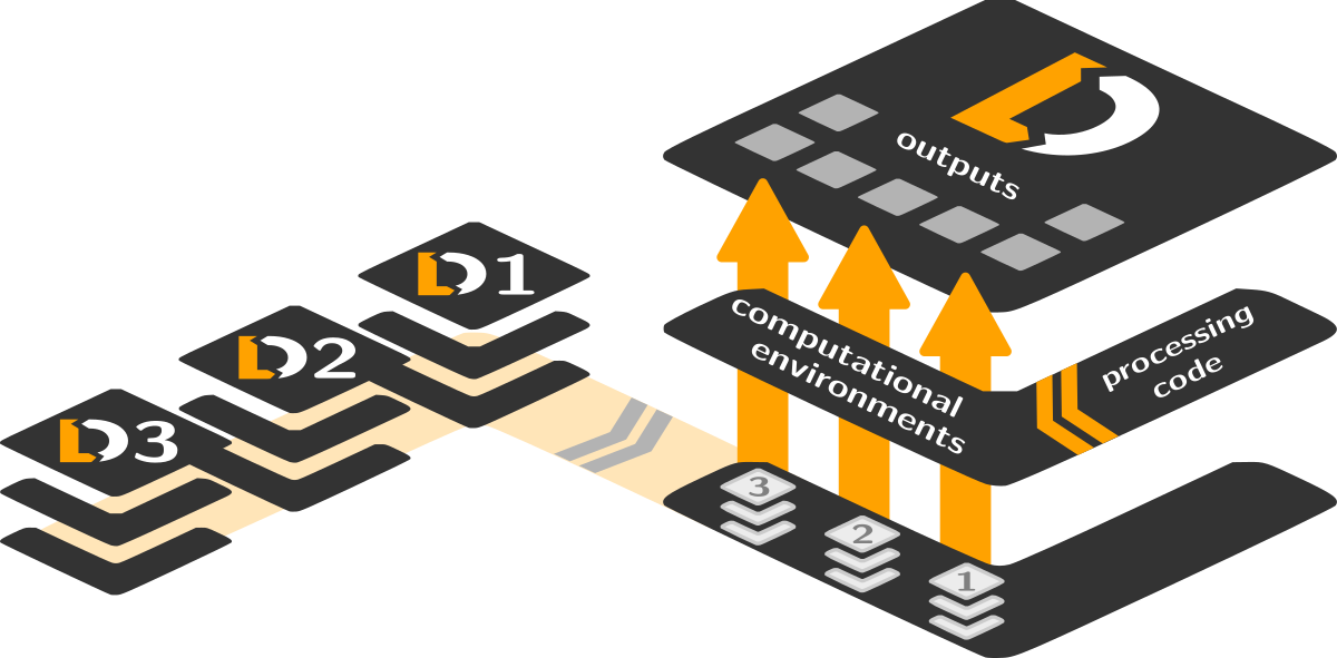
The figure above shows a schematic depiction of this comprehensive tracking. The dataset on the right tracks the state of three other dataset with input data. From those DataLad can automatically obtain any required input files for a computation which is implemented in code that is also tracked in this dataset. This code is executed by DataLad in a computational environment that is also tracked in the same dataset in the form of a container image file. From this comprehensive set of inputs the outputs are computed, and are also captured by DataLad in the same dataset.
In this lesson we will create two such datasets that represent two major components of any imaging study: 1) data conversion from raw DICOM format, and 2) data analysis for answering a specific research question. While the involved data files, code, computational environments will differ between these steps, the overall principle of comprehensive input and output capture is a common aspects shared between the two.
Modular Study Components
Imaging studies tend to involve rather complex, multi-step analyses. It is common that a single dataset is analyzed in multiple ways that in turn require different types of preprocessing. Accurate presentation of methods and results in a publication a precise understanding what exactly was done to which variant of data to produce a particular result. However, it can be very challenging to maintain this kind of awareness, especially in long-running projects that involve multiple researchers or even groups with non-overlapping responsibilities.
With DataLad’s dataset-subdataset linkage it is fairly straightforward to structure data processing in a study in modular units that enable standalone publication of intermediate steps and effortless re-use of (carefully validated) computational results.
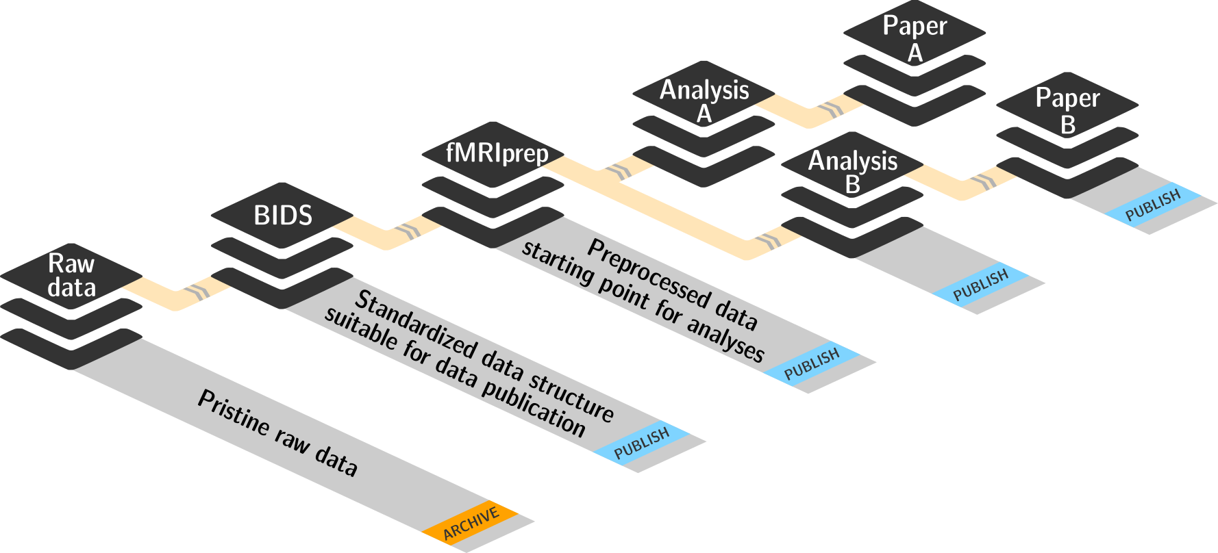
The above figure depicts a typical structure of data processing in an imaging study, going from acquired raw data, to a converted and standardized form, to preprocessed data, to one or more analysis implementations, to the respective publications. Key aspect here is that each of these steps is represented by a DataLad dataset that comprehensively tracks all inputs and outputs of a given step using the features described in the previous section. Each dataset can in turn be input to one or more additional data processing steps. While a single dataset only tracks its immediate inputs, DataLad is capable of resolving any input dependencies recursively across all subdataset levels (subdatasets of subdatasets of …). This makes it possible to discover the precise identity of data, code, and computational environments for any underlying computation – even years after a study was completed (given that each involved dataset was archived). Each modular component only has to be archived once, because it captures all states of its own evolution.
The two datasets created in this lesson represent two of those modular components: 1) imaging data in a standardized (BIDS) format, and 2) the outputs of an analysis (that includes a preprocessing step), where the second component is built atop the first component using its outputs as inputs for an analysis.
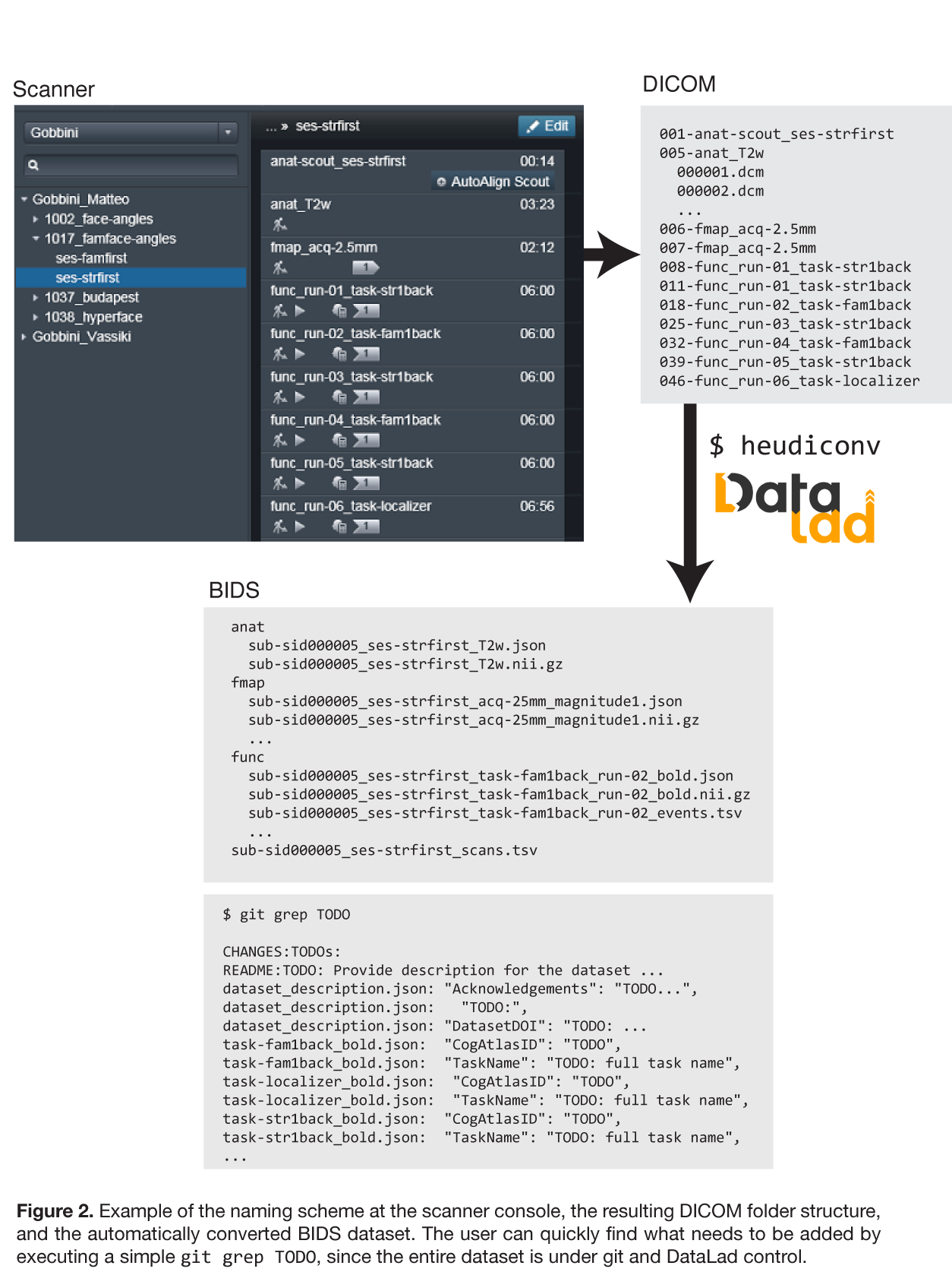
Facilitate Data Structure Standardization
Our analysis will benefit from a standardization effort that was performed at the time of data acquisition. The metadata of the input DICOM images already contain all necessary information to identify the purpose of individual scans and encode essential properties into the filenames used in a BIDS-compliant dataset. The following figure illustrates how this critical information can be encoded into the acquisition protocol names at a scanner console when setting up a new study, by following the ReproIn naming conventions.
Prepare the Data for Analysis
Before analyzing imaging data, we typically have to convert them from their original DICOM format into NIfTI files.
The data we are working with already follows the ReproIn naming conventions, and the HeuDiConv converter can use this information to automatically create a BIDS-compliant dataset for us.
We gain a lot here by adopting the BIDS standard. Up front, it saves us the effort of creating an ad-hoc directory structure. But more importantly, by structuring our data in a standard way (and an increasingly common one), it opens up possibilities for us to easily feed our dataset into existing analysis pipelines and tools.
Our first goal is to convert our DICOM data into a DataLad dataset in BIDS format.
Task: Create a new DataLad dataset called
localizer_scansUse the datalad create command
Solution
% datalad create localizer_scans
We now have the new dataset in the localizer_scans/ directory. We will change
into this directory so that all further commands will be able to use relative
paths.
% cd localizer_scans
Advantages of Relative Path Specification
In many cases, it does not matter whether one uses absolute vs relative paths, but when it comes to portability, it has a great impact. Using relative paths makes it possible to move a dataset to another folder on your system (or give it to a colleague using a different computer) and still have everything intra-connected and working as it should.
When using DataLad, it is best to always run scripts from the root directory of the dataset — and also code all scripts to use paths that are relative to this root directory. For this to work, a dataset must contain all of the inputs of a processing step (all code, all data).
That means that we should add the raw DICOM files to our dataset. In our case,
these DICOMs are already available in a DataLad dataset from
GitHub that we can
add as a subdataset to our localizer_scans dataset.
Task: Add DICOM data as a subdataset in
inputs/rawdataUse the datalad install command. Make sure to identify the
localizer_scansdataset (the current directory) as the dataset to operate on in order to register the DICOMs as a subdataset (and not simply downloaded as a standalone dataset). Then, use the datalad subdatasets command to verify the result.Solution
% datalad install --dataset . --source https://github.com/datalad/example-dicom-functional.git inputs/rawdata
% datalad subdatasets
Working With Containers
Any software you are using (and at any step) has the potential to have bugs/errors/horrifying-gremlins — and arguably already does, you just may not know it yet. Hence we take extra care to know exactly what software we are using and that we can go back to it at a later stage, should we have the need to investigate an issue.
Containerized computational environments are a great way to handle this problem. DataLad (via its datalad-container extension) provides support for using and managing such environments for data processing. We can add an image of a computational environment to a DataLad dataset (just like any other) file, so we know exactly what we are using and where to get it again in the future.
A ready-made singularity container with the HeuDiConv DICOM converter
(~160 MB) is available from singularity-hub at:
shub://ReproNim/ohbm2018-training:heudiconvn (a local copy is available at
~/images/heudiconv.simg in the training VM).
Task: Add the HeuDiConv container to the dataset
Use the datalad containers-add command to add this container under the name
heudiconv. Then use the datalad containers-list command to verify that everything worked.Solution
% # regular call
% # datalad containers-add heudiconv --url shub://ReproNim/ohbm2018-training:heudiconvn
% # BUT in the training VM do this to save on downloads
% datalad containers-add heudiconv --url ~/images/heudiconv.simg \
      --call-fmt 'singularity exec {img} {cmd}'
% datalad containers-list
Our dataset now tracks all input data and the computational environment for the DICOM conversion. This means that we have a complete record of all components (thus far) in this one dataset that we can reference via relative paths from the dataset root. This is a good starting point for conducting a portable analysis.
datalad run and datalad containers-run (provided by the datalad-container extension) allow a user to run arbitrary shell commands and capture the output in a dataset. By design, both commands behave nearly identically. The primary difference is that datalad run executes commands in the local environment, whereas datalad containers-run executes commands inside of a containerized environment. Here, we will use the latter.
Task: Convert DICOM using HeuDiConv from the container
An appropriate HeuDiConv command looks like this:
heudiconv -f reproin -s 02 -c dcm2niix -b -l "" --minmeta -a . \
    -o /tmp/heudiconv.sub-02 --files inputs/rawdata/dicoms
It essentially tells it to use the ReproIn heuristic to convert the DICOMs using the subject identifier
02, with the DICOM converterdcm2niix, into the BIDS format. The last argument is the directory containing the DICOMs.Run this command using datalad containers-run, making sure to include a meaningful commit message, so that the results of this command are saved with a meaningful context. If anything goes wrong when running the command, remember that you can use
git reset --hardon the dataset repository to throw away anything that is not yet committed.Once done, use the datalad diff command to compare the dataset to the previous saved state (
HEAD~1) to get an instant summary of the changes.Solution
It is sufficient to prefix the original command line call with
datalad containers-run.% datalad containers-run -m "Convert sub-02 DICOMs into BIDS" \ --container-name heudiconv \ heudiconv -f reproin -s 02 -c dcm2niix -b -l "" --minmeta -a . \ -o /tmp/heudiconv.sub-02 --files inputs/rawdata/dicoms % datalad diff --revision HEAD~1It is not strictly necessary to specify the name of the container to be used. If there is only one container known to a dataset, datalad containers-run is clever enough to use that one.
You can now confirm that a NIfTI file has been added to the dataset and that its name is compliant with the BIDS standard. Information such as the task-label has been automatically extracted from the imaging sequence description.
There is only one thing missing before we can analyze our functional
imaging data: we need to know what stimulation was done at which point during
the scan. Thankfully, the data was collected using an implementation that
exported this information directly in the BIDS events.tsv format. The
file came with our DICOM dataset and can be found at
inputs/rawdata/events.tsv. All we need to do is copy it to the right location
under the BIDS-mandated name.
We can use cp to do this easily, but the copying step itself would not be
entered into the dataset’s history and thus the file would be added with no
indication of where it came from. A good commit message can help with that, but
what would be even better is to run cp using datalad run to capture this
information.
Task: Copy the event.tsv file to its correct location via
runBIDS requires that this file be located at
sub-02/func/sub-02_task-oneback_run-01_events.tsv. Use the datalad run command to execute thecpcommand to implement this step. This time, however, use the options--inputand--outputto inform datalad run what files need to be available and what locations need to be writeable for this command.In order to avoid duplication, datalad run supports placeholder labels that you can use in the command specification itself.
Use
git logto investigate what information DataLad captured about this command’s execution.Solution
Prefix the original command line call with
datalad run -m "<some message>" --input <input file> --output <output file>and replace those files in the original command by{inputs}and{outputs}respectively.% datalad run -m "Import stimulation events" \ --input inputs/rawdata/events.tsv \ --output sub-02/func/sub-02_task-oneback_run-01_events.tsv \ cp {inputs} {outputs} % git log -p
We are now done with the data preparation. We have the skeleton of a BIDS-compliant dataset that contains all data in the right format and using the correct file names. In addition, the computational environment used to perform the DICOM conversion is tracked, as well as a separate dataset with the input DICOM data. This means we can trace every single file in this dataset back to its origin, including the commands and inputs used to create it.
This dataset is now ready. It can be archived and used as input for one or more analyses of any kind. Let’s leave the dataset directory now:
% cd ..
A Reproducible GLM Demo Analysis
With our raw data prepared in BIDS format, we can now conduct an analysis.
We will implement a very basic first-level GLM analysis using FSL that runs
in just a few minutes. We will follow the same principles that we already
applied when we prepared the localizer_scans dataset: the complete capture of
all inputs, computational environments, code, and outputs.
Importantly, we will conduct our analysis in a new dataset. The raw
localizer_scans dataset is suitable for many different analysis that can all
use that dataset as input. In order to avoid wasteful duplication and to improve
the modularity of our data structures, we will merely use the localizer_scans
dataset as an input, but we will not modify it in any way.
Task: Create a new DataLad dataset called
glm_analysisUse the datalad create command. Then change into the root directory of the newly created dataset.
Solution
% datalad create glm_analysis
% cd glm_analysis
Following the same logic and commands as before, we will add the
localizer_scans dataset as a subdataset of the new glm_analysis dataset to
enable comprehensive tracking of all input data within the analysis dataset.
Task: Add
localizer_scansdata as a subdataset ininputs/rawdataUse the datalad install command. Make sure to identify the analysis dataset (the current directory) as the dataset to operate on in order to register the
localizer_scansdataset as a subdataset (and not just as a standalone dataset). Then, use the datalad subdatasets command to verify the result.Solution
% datalad install --dataset . --source ../localizer_scans inputs/rawdata
% datalad subdatasets
Regarding the layout of this analysis dataset, we unfortunately cannot yet rely on automatic tools and a comprehensive standard (but such guidelines are actively being worked on). However, DataLad nevertheless aids efforts to bring order to the chaos. Anyone can develop their own ideas on how a dataset should be structured and implement these concepts in dataset procedures that can be executed using the datalad run-procedure command.
Here we are going to adopt the YODA principles: a set of simple rules on how to
structure analysis dataset. You can learn more about YODA at OHBM poster 2046
(YODA: YODA’s organigram on data analysis). But here, the only relevant aspect
is that we want to keep all analysis scripts in the code/ subdirectory of
this dataset. We can get a readily configured dataset by running the YODA
setup procedure:
Task: Run the
setup_yoda_datasetprocedureUse the datalad run-procedure command. Check what has changed in the dataset.
Solution
% datalad run-procedure setup_yoda_dataset
Before we can fire up FSL for our GLM analysis, we need two pieces of custom code:
-
a small script that can convert BIDS events.tsv files into the EV3 format that FSL can understand, available at https://raw.githubusercontent.com/myyoda/ohbm2018-training/master/section23/scripts/events2ev3.sh
-
an FSL analysis configuration template script available at https://raw.githubusercontent.com/myyoda/ohbm2018-training/master/section23/scripts/ffa_design.fsf
Any custom code needs to be tracked if we want to achieve a complete record of how an analysis was conducted. Hence we will store those scripts in our analysis dataset.
Download the Scripts and Include Them in the Analysis Dataset
Use the datalad download-url command. Place the scripts in the
code/directory under their respective names. Checkgit logto confirm that the commit message shows the URL where each script has been downloaded from.Solution
% datalad download-url --path code \
  https://raw.githubusercontent.com/myyoda/ohbm2018-training/master/section23/scripts/events2ev3.sh \
  https://raw.githubusercontent.com/myyoda/ohbm2018-training/master/section23/scripts/ffa_design.fsf
% git log
At this point, our analysis dataset contains all of the required inputs. We only have to run our custom code to produce the inputs in the format that FSL expects. First, let’s convert the events.tsv file into EV3 format files.
Task: Run the converter script for the event timing information
Use the datalad run command to execute the script at
code/events2ev3.sh. It requires the name of the output directory (usesub-02) and the location of the BIDS events.tsv file to be converted. Use the--inputand--outputoptions to let DataLad automatically manage these files for you. Important: The subdataset does not actually have the content for the events.tsv file yet. If you use--inputcorrectly, DataLad will obtain the file content for you automatically. Check the output carefully, the script is written in a sloppy way that will produce some output even when things go wrong. Each generated file must have three numbers per line.Solution
% datalad run -m 'Build FSL EV3 design files' \
      --input inputs/rawdata/sub-02/func/sub-02_task-oneback_run-01_events.tsv \
      --output 'sub-02/onsets' \
      bash code/events2ev3.sh sub-02 {inputs}
Now we’re ready for FSL! And since FSL is certainly not a simple, system
program, we will again use it in a container and add that container to this
analysis dataset. A ready-made container with FSL (~260 MB) is available from
shub://ReproNim/ohbm2018-training:fsln (a local copy is available at
~/images/fsl.simg in the training VM).
Task: Add a container with FSL
Use the datalad containers-add command to add this container under the name
fsl. Then use the datalad containers-list command to verify that everything worked.Solution
% # regular call
% datalad containers-add fsl --url shub://ReproNim/ohbm2018-training:fsln
% # BUT in the training VM do this to save on downloads
% datalad containers-add fsl --url ~/images/fsl.simg \
      --call-fmt 'singularity exec {img} {cmd}'
%
% datalad containers-list
With this we have completed the analysis setup. At such a milestone it can be
useful to label the state of a dataset that can be referred to later on. Let’s
add the label ready4analysis here.
% datalad save --version-tag ready4analysis
All we have left is to configure the desired first-level GLM analysis with FSL.
The following command will create a working configuration from the template we
stored in code/. It uses the arcane, yet powerful sed editor. We will again
use datalad run to invoke our command so that we store in the history
how this template was generated (so that we may audit, alter, or regenerate
this file in the future — fearlessly).
datalad run \
    -m "FSL FEAT analysis config script" \
    --output sub-02/1stlvl_design.fsf \
    bash -c 'sed -e "s,##BASEPATH##,{pwd},g" -e "s,##SUB##,sub-02,g" \
        code/ffa_design.fsf > {outputs}'
The command that we will run now in order to compute the analysis results is a
simple feat sub-02/1stlvl_design.fsf. However, in order to achieve the most
reproducible and most portable execution, we should tell the datalad
containers-run command what the inputs and outputs are. DataLad will then be
able to obtain the required NIfTI time series file from the localizer_scans
raw subdataset.
Please run the following command as soon as possible; it takes around 5 minutes to complete on an average system.
datalad containers-run --container-name fsl -m "sub-02 1st-level GLM" \
    --input sub-02/1stlvl_design.fsf \
    --input sub-02/onsets \
    --input inputs/rawdata/sub-02/func/sub-02_task-oneback_run-01_bold.nii.gz \
    --output sub-02/1stlvl_glm.feat \
    feat {inputs[0]}
Once this command finishes, DataLad will have captured the entire FSL output, and the dataset will contain a complete record all the way from the input BIDS dataset to the GLM results (which, by the way, performed an FFA localization on a real BOLD imaging dataset, take a look!). The BIDS subdataset in turn has a complete record of all processing down from the raw DICOMs onwards.
Get Ready for the Afterlife
Once a study is complete and published it is important to archive data and
results, for example, to be able to respond to inquiries from readers of an
associated publication. The modularity of the study units makes this
straightforward and avoid needless duplication. We now that the raw data for
this GLM analysis is tracked in its own dataset (localizer_scans) that only
needs to be archived once, regardless of how many analyses use it as input.
This means that we can “throw away” this subdataset copy within this
analysis dataset. DataLad can re-obtain the correct version at any point in
the future, as long as the recorded location remains accessible.
Task: Verify that the
localizer_scanssubdataset is unmodified and uninstall itUse the datalad diff command and
git logto verify that the subdataset is in the same state as when it was initially added. Then use datalad uninstall to delete it.Solution
% datalad diff -- inputs
% git log -- inputs
% datalad uninstall --dataset . inputs --recursive
Before we archive these analysis results, we can go one step further and verify
their computational reproducibility. DataLad provides a rerun command that is
capable of “replaying” any recorded command. The following command we
re-execute the FSL analysis (the command that was recorded since we tagged the
dataset as “ready4analysis”). It will record the recomputed results in a
separate Git branch named “verify” of the dataset. We can then automatically
compare these new results to the original ones in the “master” branch. We
will see that all outputs can be reproduced in bit-identical form. The only
changes are observed in log files that contain volatile information, such
as time steps.
# rerun FSL analysis from scratch (~5 min)
% datalad rerun --branch verify --onto ready4analysis --since ready4analysis
% # check that we are now on the new `verify` branch
% git branch
% # compare which files have changes with respect to the original results
% git diff master --stat
% # switch back to the master branch and remove the `verify` branch
% git checkout master
% git branch -D verify
Key Points
we can implement a complete imaging study using DataLad datasets to represent units of data processing
each unit comprehensively captures all inputs and data processing leading up to it
this comprehensive capture facilitates re-use of units, and enables computational reproducibility
carefully validated intermediate results (captured as a DataLad dataset) are a candidate for publication with minimal additional effort
the outcome of this demo is available as a demo DataLad dataset from GitHub